World Hapiness

Which factors contribute to the hapiness of a nation? 2022 is coming, let us look back the global hapiness over time!

In this post, we are studying the World Hapiness Report dataset, which is a landmark survey of the state of global happiness. The dataset is useful for interdisciplinary fields, ranging from economics, public health to psycholgy and development policy. The dataset contains 2 parts, the world hapiness report over time and the report for the year 2021.

import numpy as np
import pandas as pd
import matplotlib.pyplot as plt
import seaborn as sns
import sklearn.linear_model

import matplotlib.gridspec as gs
import seaborn as sns

df = pd.read_csv("world-happiness-report.csv")
df.head()

	Country name	year	Life Ladder	Log GDP per capita	Social support	Healthy life expectancy at birth	Freedom to make life choices	Generosity	Perceptions of corruption	Positive affect	Negative affect
0	Afghanistan	2008	3.724	7.370	0.451	50.80	0.718	0.168	0.882	0.518	0.258
1	Afghanistan	2009	4.402	7.540	0.552	51.20	0.679	0.190	0.850	0.584	0.237
2	Afghanistan	2010	4.758	7.647	0.539	51.60	0.600	0.121	0.707	0.618	0.275
3	Afghanistan	2011	3.832	7.620	0.521	51.92	0.496	0.162	0.731	0.611	0.267
4	Afghanistan	2012	3.783	7.705	0.521	52.24	0.531	0.236	0.776	0.710	0.268

df2021 = pd.read_csv("world-happiness-report-2021.csv")
df2021.head()

	Country name	Regional indicator	Ladder score	Standard error of ladder score	upperwhisker	lowerwhisker	Logged GDP per capita	Social support	Healthy life expectancy	Freedom to make life choices	Generosity	Perceptions of corruption	Ladder score in Dystopia	Explained by: Log GDP per capita	Explained by: Social support	Explained by: Healthy life expectancy	Explained by: Freedom to make life choices	Explained by: Generosity	Explained by: Perceptions of corruption	Dystopia + residual
0	Finland	Western Europe	7.842	0.032	7.904	7.780	10.775	0.954	72.0	0.949	-0.098	0.186	2.43	1.446	1.106	0.741	0.691	0.124	0.481	3.253
1	Denmark	Western Europe	7.620	0.035	7.687	7.552	10.933	0.954	72.7	0.946	0.030	0.179	2.43	1.502	1.108	0.763	0.686	0.208	0.485	2.868
2	Switzerland	Western Europe	7.571	0.036	7.643	7.500	11.117	0.942	74.4	0.919	0.025	0.292	2.43	1.566	1.079	0.816	0.653	0.204	0.413	2.839
3	Iceland	Western Europe	7.554	0.059	7.670	7.438	10.878	0.983	73.0	0.955	0.160	0.673	2.43	1.482	1.172	0.772	0.698	0.293	0.170	2.967
4	Netherlands	Western Europe	7.464	0.027	7.518	7.410	10.932	0.942	72.4	0.913	0.175	0.338	2.43	1.501	1.079	0.753	0.647	0.302	0.384	2.798

df.rename(columns={'Country name': 'Country'}, inplace=True)
df2021.rename(columns={'Country name': 'Country'}, inplace=True)

Explanatory data analysis for the year 2021

c1 = "mediumturquoise"
c2 = "lightpink"
c3 = "sandybrown"

high_c = c1
low_c = c2

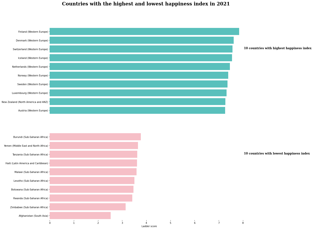
Countries with the highest and lowest happiness index in 2021

#top 10 and lowesttom 10 countries in 2021 report
fig= plt.figure(figsize=(15,15))
g=gs.GridSpec(ncols=1, nrows=2, figure=fig)
plt.suptitle("Countries with the highest and lowest happiness index in 2021", family='Serif', weight='bold', size=20)
ax1=plt.subplot(g[0,0])

top_10=df2021.head(10)
lowest_10= df2021.tail(10)
ax1=sns.barplot(data=top_10, x=top_10['Ladder score'],
                y=top_10['Country']+ " (" + top_10['Regional indicator'] + ")", color = c1)
#ax1.set_xlabel('')
ax1.xaxis.set_visible(False)
ax1.annotate(" 10 countries with highest happiness index",xy=(8,2), family='Serif', weight='bold', size=12)
ax2=plt.subplot(g[1,0], sharex=ax1)
ax2=sns.barplot(data=lowest_10, x=lowest_10['Ladder score'],
                y=lowest_10['Country']+ " (" + lowest_10['Regional indicator'] + ")",  color = c2)
ax2.annotate(" 10 countries with lowest happiness index",xy=(8,2), family='Serif', weight='bold', size=12)
for s in ['left','right','top','bottom']:
    ax1.spines[s].set_visible(False)
    ax2.spines[s].set_visible(False)

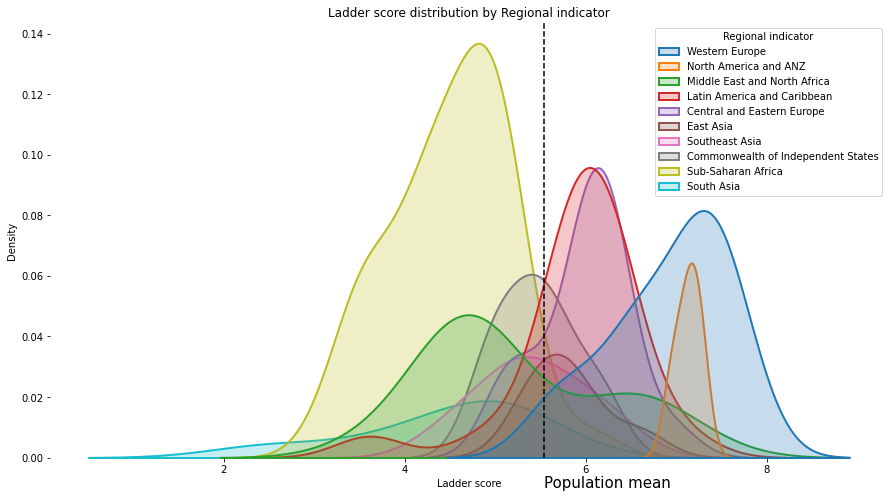
Ladder score distribution by Regional indicator

fig=plt.figure(figsize=(15,8))
plt.title("Ladder score distribution by Regional indicator")
sns.kdeplot(df2021['Ladder score'], fill=True,hue=df2021['Regional indicator'], shade=True, linewidth=2, multiple='layer')
plt.axvline(df2021['Ladder score'].mean(), c='black',ls='--')
plt.text(x=df2021['Ladder score'].mean(),y=-0.01,s='Population mean', size=15)
for s in ['left','right','top','bottom']:
    plt.gca().spines[s].set_visible(False)

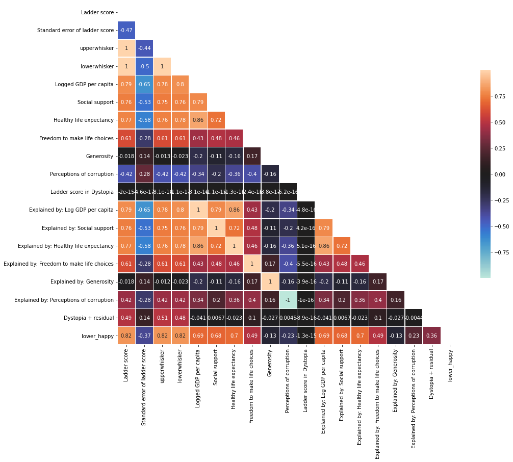
Correlaztion analysis for the year 2021

corr = df2021.corr()
mask = np.zeros_like(corr)
mask[np.triu_indices_from(mask)] = True
plt.figure(figsize=(15,15))
sns.heatmap(corr, mask=mask, center=0, annot=True,
            square=True, linewidths=.5, cbar_kws={"shrink": .5})
plt.show()

#refined
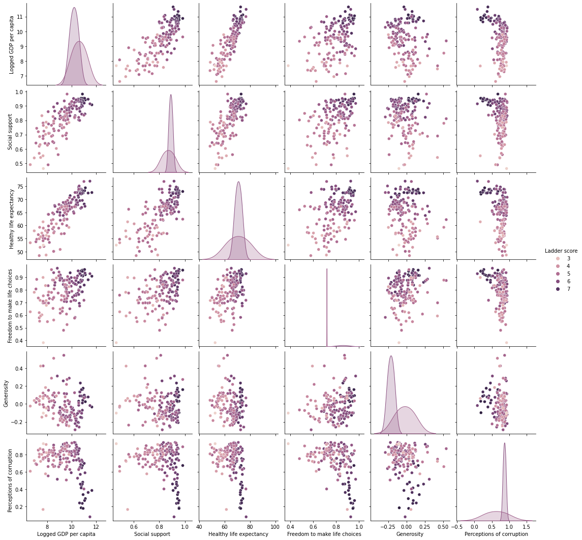
continuous = ['Logged GDP per capita',
 'Social support',
 'Healthy life expectancy',
 'Freedom to make life choices',
 'Generosity',
 'Perceptions of corruption']

sns.pairplot(df2021, vars = continuous,  hue = 'Ladder score')

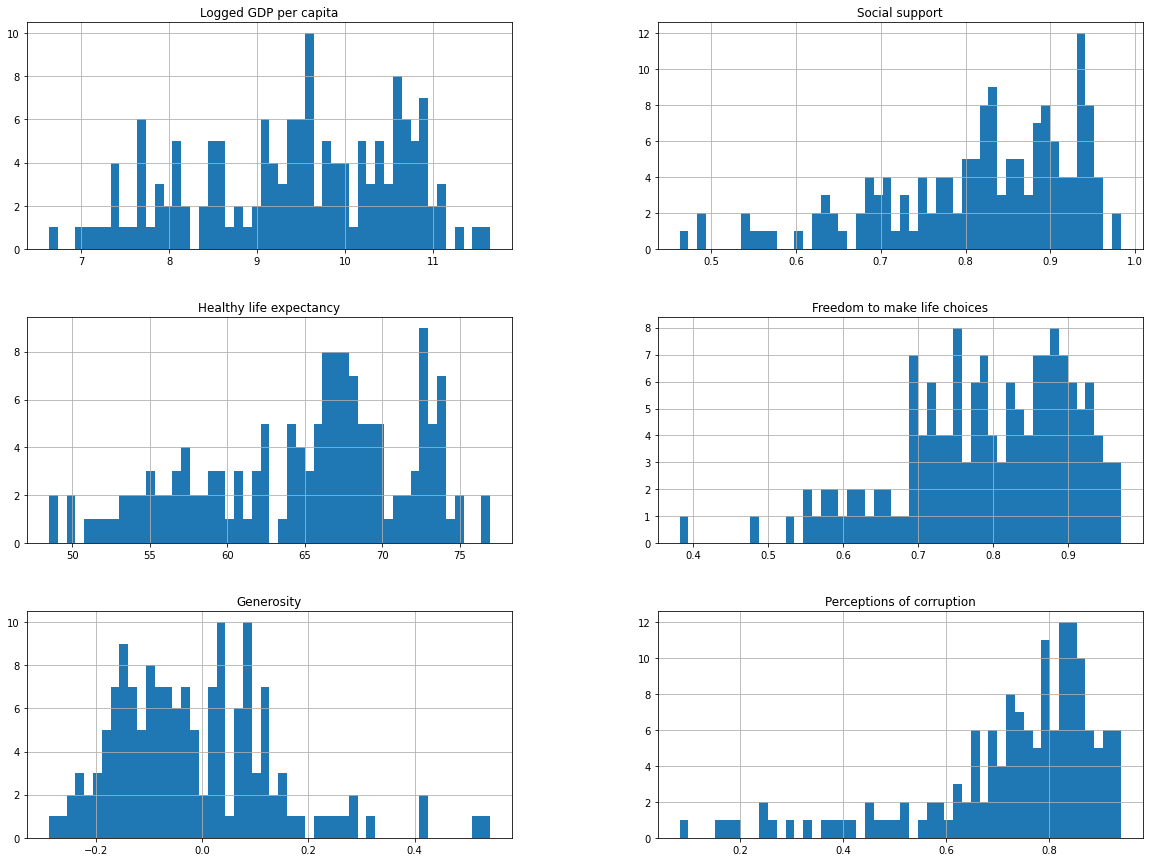
df2021[continuous].hist(bins=50, figsize=(20,15))
plt.show()

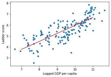
Correlation GDP-Hapiness index

# get GDP for the x-axis and Life Satisfaction for the y-axis
X = df2021['Logged GDP per capita'].values.reshape(-1, 1)
y = df2021['Ladder score'].values.reshape(-1, 1)
X.shape, y.shape

((149, 1), (149, 1))

# Select a Linear Model
model = sklearn.linear_model.LinearRegression()
# Train the Model
model.fit(X, y)

LinearRegression()

# let's visualize our model, because it's a linear one, we can plot it using two points
X = [[7], [11]]
y_hat = model.predict(X)
df2021.plot(kind='scatter', x='Logged GDP per capita', y='Ladder score')
plt.plot(X, y_hat, c='red')
plt.show()

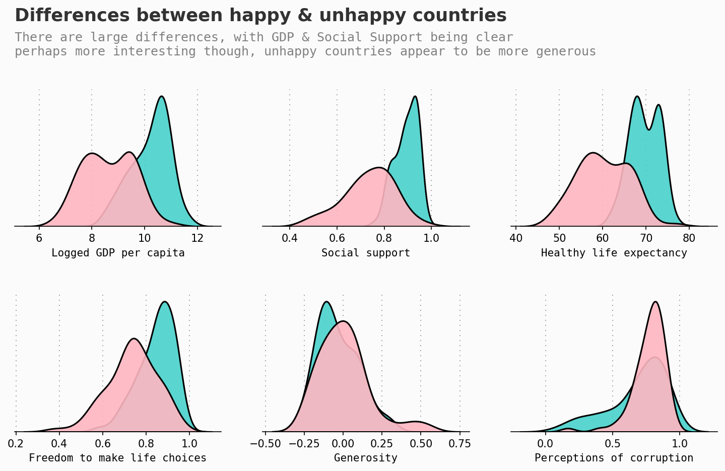
Distribution of ladder score compared to other factors

happiness_mean = df2021['Ladder score'].mean()

df2021['lower_happy'] = df2021['Ladder score'].apply(lambda x: 0 if x < happiness_mean else 1)

background_color = '#fbfbfb'
fig = plt.figure(figsize=(12, 6), dpi=150,facecolor=background_color)
gs = fig.add_gridspec(2, 3)
gs.update(wspace=0.2, hspace=0.5)


plot = 0
for row in range(0, 2):
    for col in range(0, 3):
        locals()["ax"+str(plot)] = fig.add_subplot(gs[row, col])
        locals()["ax"+str(plot)].set_facecolor(background_color)
        locals()["ax"+str(plot)].tick_params(axis='y', left=False)
        locals()["ax"+str(plot)].get_yaxis().set_visible(False)
        locals()["ax"+str(plot)].set_axisbelow(True)
        for s in ["top","right","left"]:
            locals()["ax"+str(plot)].spines[s].set_visible(False)
        plot += 1

plot = 0

Yes = df2021[df2021['lower_happy'] == 1]
No = df2021[df2021['lower_happy'] == 0]


 
for variable in continuous:
        sns.kdeplot(Yes[variable], ax=locals()["ax"+str(plot)], color=high_c,ec='black', shade=True, linewidth=1.5, alpha=0.9, zorder=3, legend=False)
        sns.kdeplot(No[variable],ax=locals()["ax"+str(plot)], color=low_c, shade=True, ec='black',linewidth=1.5, alpha=0.9, zorder=3, legend=False)
        locals()["ax"+str(plot)].grid(which='major', axis='x', zorder=0, color='gray', linestyle=':', dashes=(1,5))
        locals()["ax"+str(plot)].set_xlabel(variable, fontfamily='monospace')
        plot += 1
        
Xstart, Xend = ax0.get_xlim()
Ystart, Yend = ax0.get_ylim()

ax0.text(Xstart, Yend+(Yend*0.5), 'Differences between happy & unhappy countries', fontsize=17, fontweight='bold', fontfamily='sansserif',color='#323232')
ax0.text(Xstart, Yend+(Yend*0.25), 'There are large differences, with GDP & Social Support being clear\nperhaps more interesting though, unhappy countries appear to be more generous', fontsize=12, fontweight='light', fontfamily='monospace',color='gray')

plt.show()

findfont: Font family ['sansserif'] not found. Falling back to DejaVu Sans.

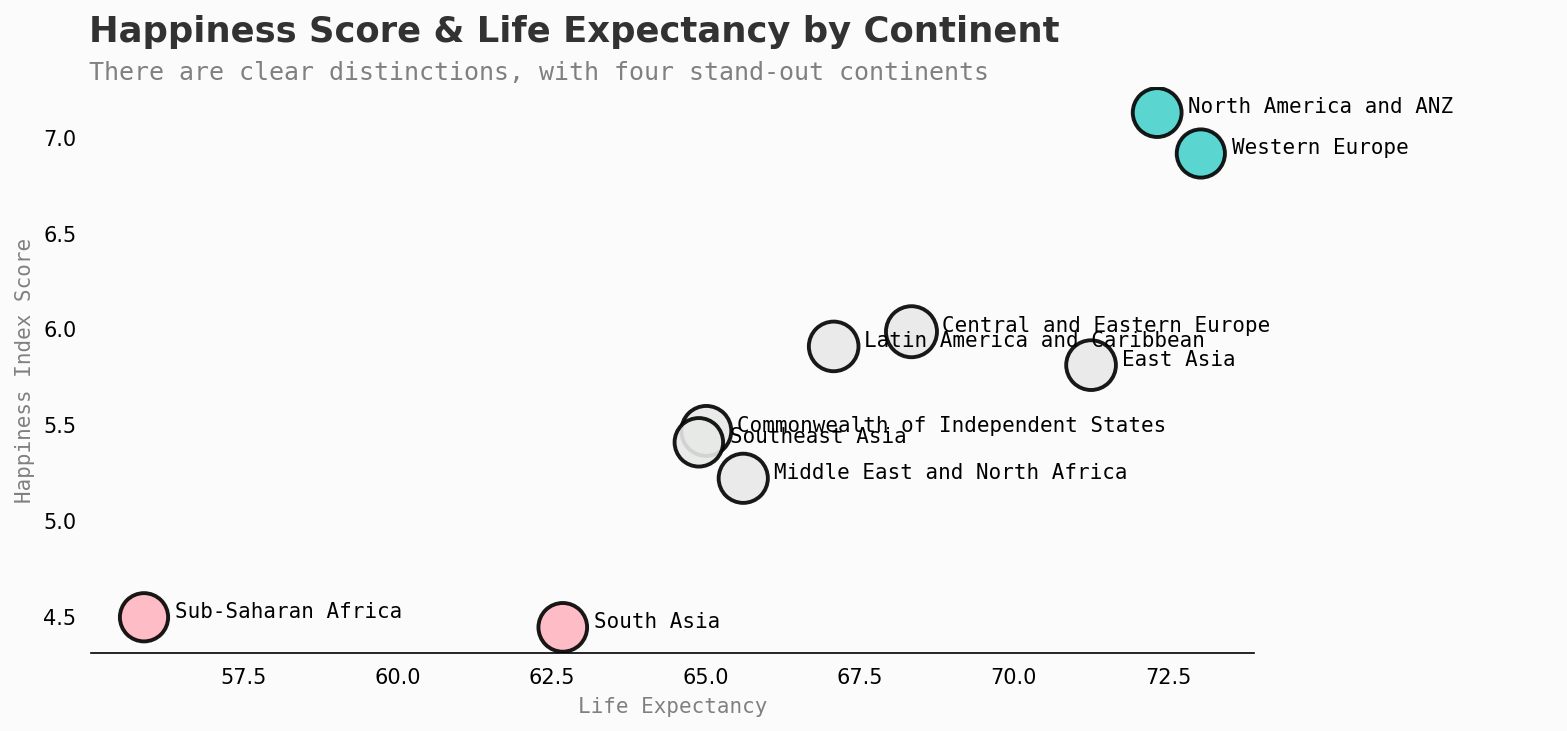
A continental view

continent_score = df2021.groupby('Regional indicator')['Healthy life expectancy','Logged GDP per capita','Perceptions of corruption','Freedom to make life choices','Ladder score'].mean().reset_index()

background = "#fbfbfb"

fig, ax = plt.subplots(1,1, figsize=(10, 5),dpi=150)
fig.patch.set_facecolor(background) # figure background color

cmap = [c2,c1]


color_map = ['#e7e9e7' for _ in range(10)]
color_map[9] =  c1 # color highlight
color_map[5] =  c1
color_map[8] =  c2
color_map[6] =  c2


ax.set_facecolor(background)
sns.scatterplot(data=continent_score, x=continent_score['Healthy life expectancy'], y=continent_score['Ladder score'],hue=continent_score['Regional indicator'], alpha=0.9,ec='black',palette=color_map,size=df2021["Ladder score"], legend=False, sizes=(5, 600))

ax.set_xlabel("Life Expectancy",fontfamily='monospace',color='gray')
ax.set_ylabel("Happiness Index Score",fontfamily='monospace',color='gray')
ax.tick_params(axis = 'both', which = 'major', labelsize = 10)

for s in ["top","right","left"]:
    ax.spines[s].set_visible(False)
    
ax.text(55,7.5,'Happiness Score & Life Expectancy by Continent',fontfamily='sansserif',fontweight='normal',fontsize=17,weight='bold',color='#323232')
ax.text(55,7.3,'There are clear distinctions, with four stand-out continents',fontfamily='monospace',fontweight='light',fontsize=12,color='gray')



L = ax.legend(frameon=False,loc="upper center", bbox_to_anchor=(1.25, 0.8), ncol= 1)
plt.setp(L.texts, family='monospace')
L.get_frame().set_facecolor('none')


ax.tick_params(axis='both', which='both',left=False, bottom=False,labelbottom=True) 

for i, txt in enumerate(continent_score['Regional indicator']):
    ax.annotate(txt, (continent_score['Healthy life expectancy'][i]+0.5, continent_score['Ladder score'][i]),fontfamily='monospace')


    
plt.show()

/usr/local/lib/python3.7/dist-packages/ipykernel_launcher.py:1: FutureWarning: Indexing with multiple keys (implicitly converted to a tuple of keys) will be deprecated, use a list instead.
  """Entry point for launching an IPython kernel.
No handles with labels found to put in legend.

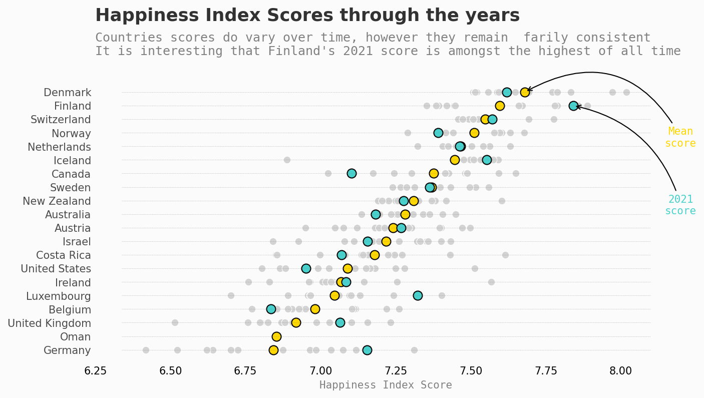
Happiness index over time

background = "#fbfbfb"
fig, ax = plt.subplots(1,1, figsize=(10, 5),dpi=150)
fig.patch.set_facecolor(background) # figure background color
ax.set_facecolor(background)

# Reduced list as too many to show all at once 
top_list_ = df.groupby('Country')['Life Ladder'].mean().sort_values(ascending=False).reset_index()[:20].sort_values(by='Life Ladder',ascending=True)


plot = 1
for country in top_list_['Country']:
    mean = df[df['Country'] == country].groupby('Country')['Life Ladder'].mean()
    # historic scores
    sns.scatterplot(data=df[df['Country'] == country], y=plot, x='Life Ladder',color='lightgray',s=50,ax=ax)
    # mean score
    sns.scatterplot(data=df[df['Country'] == country], y=plot, x=mean,color='gold',ec='black',linewidth=1,s=75,ax=ax)
    #2021 score
    sns.scatterplot(data=df2021[df2021['Country'] == country], y=plot, x='Ladder score',color=c1,ec='black',linewidth=1,s=75,ax=ax)   
    plot += 1


ax.set_yticks(top_list_.index+1)
ax.set_yticklabels(top_list_['Country'][::-1], fontdict={'horizontalalignment': 'right'}, alpha=0.7)
ax.tick_params(axis=u'both', which=u'both',length=0)
ax.set_xlabel("Happiness Index Score",fontfamily='monospace',color='gray')


for s in ['top','right','bottom','left']:
    ax.spines[s].set_visible(False)
    
Xstart, Xend = ax.get_xlim()
Ystart, Yend = ax.get_ylim()

ax.hlines(y=top_list_.index+1, xmin=Xstart, xmax=Xend, color='gray', alpha=0.5, linewidth=.3, linestyles='--')
ax.set_axisbelow(True)
ax.text(6.25, Yend+4.3, 'Happiness Index Scores through the years', fontsize=17, fontweight='bold', fontfamily='sansserif',color='#323232')
ax.text(6.25, Yend+0.75,
'''
Countries scores do vary over time, however they remain  farily consistent
It is interesting that Finland's 2021 score is amongst the highest of all time
''', fontsize=12, fontweight='light', fontfamily='monospace',color='gray')

plt.annotate('2021\nscore', xy=(7.842, 19), xytext=(8.2, 11),
             arrowprops=dict(facecolor='steelblue',arrowstyle="->",connectionstyle="arc3,rad=.3"), fontsize=10,fontfamily='monospace',ha='center', color=c1)

plt.annotate('Mean\nscore', xy=(7.6804, 20), xytext=(8.2, 16),
             arrowprops=dict(facecolor='steelblue',arrowstyle="->",connectionstyle="arc3,rad=.5"), fontsize=10,fontfamily='monospace',ha='center', color='gold')


plt.show()

A global view over time

import plotly.express as px

fig = px.choropleth(data_frame=df, locations='Country',
                    locationmode="country names",
                    color='Life Ladder',
                    animation_frame='year',
                    range_color = "",
                    #color_continuous_scale = [c2,c1])
                    color_continuous_scale = px.colors.sequential.RdBu)
fig.show()

fig.write_html("world_hapiness.html")

Regression

df.drop("year", axis=1).hist(bins=50, figsize=(20,15))
plt.show()

Create a test set

df_ = df2021[['Ladder score',
       'Standard error of ladder score', 'upperwhisker', 'lowerwhisker',
       'Logged GDP per capita', 'Social support', 'Healthy life expectancy',
       'Freedom to make life choices', 'Generosity',
       'Perceptions of corruption']]

Transformation pipelines

from sklearn.pipeline import Pipeline
from sklearn.preprocessing import StandardScaler

num_pipeline = Pipeline([
    ('std_scaler', StandardScaler())
])

df_ = num_pipeline.fit_transform(df_)
df_.shape

(149, 10)

from sklearn.model_selection import train_test_split
train_set, test_set = train_test_split(df_, test_size=0.2, random_state=42)

train_set.shape, test_set.shape

((119, 10), (30, 10))

Select and Train Model

Linear Model

from sklearn.linear_model import LinearRegression
from sklearn.metrics import mean_squared_error

lin_reg = LinearRegression()

lin_reg.fit(X=train_set[:, 1:], y=train_set[:,0])

LinearRegression()

from sklearn.metrics import mean_squared_error

predictions = lin_reg.predict(test_set[:, 1:])
lin_mse = mean_squared_error(test_set[:, 0], predictions)
lin_rmse = np.sqrt(lin_mse)
lin_rmse 

0.00031220104713910665

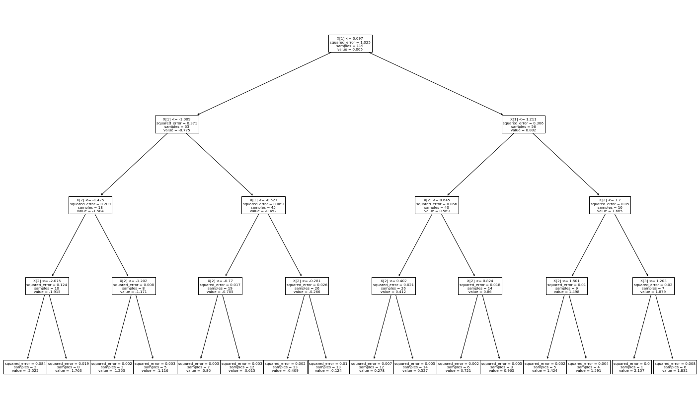
Decision Tree

from sklearn.tree import DecisionTreeRegressor

tree_reg = DecisionTreeRegressor(max_depth = 4)
tree_reg.fit(X=train_set[:, 1:], y=train_set[:,0])

DecisionTreeRegressor(max_depth=4)

predictions = tree_reg.predict(test_set[:, 1:])
lin_mse = mean_squared_error(test_set[:, 0], predictions)
lin_rmse = np.sqrt(lin_mse)
lin_rmse 

0.1019944246040892

fig = plt.figure(figsize=(25,15))
sklearn.tree.plot_tree(tree_reg)
plt.show()

Cross-Validation

from sklearn.model_selection import cross_val_score

scores = cross_val_score(estimator=tree_reg, X=train_set[:, 1:], y=train_set[:,0]
                         , scoring='neg_mean_squared_error', cv=10)

tree_rmse_scores = np.sqrt(-scores)
print("Scores:", tree_rmse_scores)
print("Mean:", tree_rmse_scores.mean())
print("Standard Deviation:", tree_rmse_scores.std())

Scores: [0.08063915 0.12074651 0.10401294 0.11853572 0.16611299 0.07206908
 0.11776827 0.13357675 0.1597485  0.25173151]
Mean: 0.13249414280237842
Standard Deviation: 0.04877781586110474

Ensemble Learning with the Random Forest

from sklearn.ensemble import RandomForestRegressor
forest_reg = RandomForestRegressor()
forest_reg.fit(X=train_set[:, 1:], y=train_set[:,0])

RandomForestRegressor()

forest_mse = mean_squared_error(y_true=test_set[:, 0], y_pred=forest_reg.predict(X=test_set[:, 1:]))
forest_rmse = np.sqrt(forest_mse)
forest_rmse

0.04082603271734864

scores = cross_val_score(estimator=forest_reg, X=train_set[:, 1:], y=train_set[:,0]
                         , scoring='neg_mean_squared_error', cv=10)
forest_rmse_scores = np.sqrt(-scores)
print("Scores:", forest_rmse_scores)
print("Mean:", forest_rmse_scores.mean())
print("Standard Deviation:", forest_rmse_scores.std()) # much better now

Scores: [0.02182252 0.0849461  0.02198475 0.07533847 0.15627785 0.05930377
 0.03977674 0.05536409 0.06649303 0.25151086]
Mean: 0.08328181891050981
Standard Deviation: 0.06690200008334836

Finetune with Grid-Search

from sklearn.model_selection import GridSearchCV

param_grid = [
    {'n_estimators': [3, 10, 30], 'max_features': [2, 4, 6, 8]},
    {'bootstrap': [False], 'n_estimators': [3, 10], 'max_features': [2, 3, 4]}
]

forest_reg = RandomForestRegressor()
grid_search = GridSearchCV(estimator=forest_reg, param_grid=param_grid, scoring='neg_mean_squared_error', cv=5, return_train_score=True, n_jobs=-1)
grid_search.fit(X=train_set[:, 1:], y=train_set[:,0])

GridSearchCV(cv=5, estimator=RandomForestRegressor(), n_jobs=-1,
             param_grid=[{'max_features': [2, 4, 6, 8],
                          'n_estimators': [3, 10, 30]},
                         {'bootstrap': [False], 'max_features': [2, 3, 4],
                          'n_estimators': [3, 10]}],
             return_train_score=True, scoring='neg_mean_squared_error')

grid_search.best_params_

{'max_features': 8, 'n_estimators': 30}

grid_search.best_estimator_

RandomForestRegressor(max_features=8, n_estimators=30)

cvres = grid_search.cv_results_

for mean_score, params in zip(cvres['mean_test_score'], cvres['params']):
    print(np.sqrt(-mean_score), params)

0.34082522900363926 {'max_features': 2, 'n_estimators': 3}
0.24008412892225006 {'max_features': 2, 'n_estimators': 10}
0.21986291868367538 {'max_features': 2, 'n_estimators': 30}
0.17776709950308564 {'max_features': 4, 'n_estimators': 3}
0.1468019626867688 {'max_features': 4, 'n_estimators': 10}
0.12742906434054158 {'max_features': 4, 'n_estimators': 30}
0.14940029641388528 {'max_features': 6, 'n_estimators': 3}
0.11440546627455518 {'max_features': 6, 'n_estimators': 10}
0.12027962076790268 {'max_features': 6, 'n_estimators': 30}
0.10803897201257359 {'max_features': 8, 'n_estimators': 3}
0.12045244766329144 {'max_features': 8, 'n_estimators': 10}
0.0991261383049853 {'max_features': 8, 'n_estimators': 30}
0.19098266384099238 {'bootstrap': False, 'max_features': 2, 'n_estimators': 3}
0.21873900029484047 {'bootstrap': False, 'max_features': 2, 'n_estimators': 10}
0.17707483768792917 {'bootstrap': False, 'max_features': 3, 'n_estimators': 3}
0.15222447554234794 {'bootstrap': False, 'max_features': 3, 'n_estimators': 10}
0.15742856042032355 {'bootstrap': False, 'max_features': 4, 'n_estimators': 3}
0.11996174232954583 {'bootstrap': False, 'max_features': 4, 'n_estimators': 10}

Randomized Search

from sklearn.model_selection import RandomizedSearchCV
from scipy.stats import randint

param_distribs = {
        'n_estimators': randint(low=1, high=200),
        'max_features': randint(low=1, high=9),
    }

forest_reg = RandomForestRegressor(random_state=42)
rnd_search = RandomizedSearchCV(forest_reg, param_distributions=param_distribs,
                                n_iter=10, cv=5, scoring='neg_mean_squared_error', random_state=42)
rnd_search.fit(X=train_set[:, 1:], y=train_set[:,0])

RandomizedSearchCV(cv=5, estimator=RandomForestRegressor(random_state=42),
                   param_distributions={'max_features': <scipy.stats._distn_infrastructure.rv_frozen object at 0x7fd1efe54250>,
                                        'n_estimators': <scipy.stats._distn_infrastructure.rv_frozen object at 0x7fd1efea9590>},
                   random_state=42, scoring='neg_mean_squared_error')

cvres = rnd_search.cv_results_
for mean_score, params in zip(cvres["mean_test_score"], cvres["params"]):
    print(np.sqrt(-mean_score), params)

0.1026364152276238 {'max_features': 7, 'n_estimators': 180}
0.11023158498480463 {'max_features': 5, 'n_estimators': 15}
0.14301237257745014 {'max_features': 3, 'n_estimators': 72}
0.10729242519657402 {'max_features': 5, 'n_estimators': 21}
0.10407094852494171 {'max_features': 7, 'n_estimators': 122}
0.14463386329172387 {'max_features': 3, 'n_estimators': 75}
0.14467805582633234 {'max_features': 3, 'n_estimators': 88}
0.10730669220705276 {'max_features': 5, 'n_estimators': 100}
0.1014822451619872 {'max_features': 8, 'n_estimators': 152}
0.14540216293970593 {'max_features': 3, 'n_estimators': 150}

feature_importances = grid_search.best_estimator_.feature_importances_
feature_importances

array([5.62869082e-04, 4.81859114e-01, 5.08040907e-01, 4.28212124e-04,
       6.71086804e-04, 4.51735910e-04, 9.18665718e-04, 1.49157615e-03,
       5.57583298e-03])